Calculating working days in excel

Calculating working days in Excel

When you want to see the total number of days your employee work in a month or in a year , you do manual calculations putting a rough estimation of how many Saturdays, Sundays and N number of holidays would be there in a period and get an approximate number of working days . Not to worry because Excel does provide you with an option to calculate the working days in excel from a particular start date to end date, excluding Saturdays ,Sundays and holidays.The function that we are going to use for this purpose is called NETWORKDAYS.INTL . 

The function returns the number of whole workdays between two dates using parameters to indicate which and how many days are weekend days. Weekend days and any days that are specified as holidays are not considered as workdays

Syntax

NETWORKDAYS.INTL(start_date, end_date, [weekend], [holidays])

The start date is the date you want to start from and end date is the date you want the working days till. Now the weekends is an optional parameter and is basically the days we don't include in the working days, it can take values like 1- for taking sat,sun as weekend , 2- Sun ,Mon etc. Holidays is again an optional parameters which is a list of non-working days.

Using the function

Now we take the example we create two list one the list of holidays in the year, list of start and end month for each date (Please note its just an example you can tweak as you like) as shown in the image below.

So now the days calculation has three parts one normal days difference i.e nothing but End Date-Start date. Now for the second column we use the function Networkdays.intl,in column I

=NETWORKDAYS.INTL(E6,F6,1)

Where E6 is the start date , F6 is the end date and 1 represents Saturday and Sunday, you can tweak it as you like it has 19 options for eg. if you are in Dubai you can use 7- where weekends are Friday and Saturday.

Notice the answers gives us 22 which is basically all the weekdays in a month. Now the next part is excluding the holidays also for that we use the formula in column J

=NETWORKDAYS.INTL(E6,F6,1,$C$6:$C$17)

The C6:C17 is nothing but the list of holidays, you can add as many as you like . Notice that in January the working days were 22 and now after removing holidays it is 20 and similarly for other months.

Use case

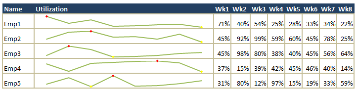
This function is really helpful for those you want to calculate the working hours in a company from a particular date . Calculating the effective utilization of the firm etc.

What-if-Analysis for Excel Part 3- Scenario Manager

What-If-Analysis - Scenario Manager

In this last session of what-if-Analysis for Excel we are going to discuss Scenario Manager. In case you missed the first two part you can use the link below to view them

For using Goal Seek in Excel use the link below -
http://manishexcel.blogspot.in/2015/09/what-if-analysis-for-excel-part-1-goal.html

For using Data Tables in Excel use the link below -

http://manishexcel.blogspot.in/2015/09/what-if-analysis-for-excel-part-2-data.html

Scenario Manager

Scenario Manager allow you to create a series of possible drivers to show in your model. The effect on Many variable on the model for different scenarios

Using Scenario Manager

The problem we are going to discuss is the same.

Where quantity is quantity sold , Unit Price is the cost to make each item , cost price is selling price . Revenues is Quantity * Cost price , CoGS(cost of goods sold) is -Quantity* Unit Price , fixed cost is some cost to produce items. Assuming we dont have any other expense or profit the

Net Profit=Revenues + CoGS+Fixed Cost

Now what we want to see is how would Net Profit change if we change other input variables and we want to store result of each change.The steps are as follows.

1.Click the Datatab, click What-if-Analysis, and choose Scenario Manager . The scenario Manager Dialog is displayed below

2.The Scenario Manager dialog box is shown below.

3. Click on Add to add scenarios.

4. Now in the box scenario name click give the name of the scenario , in our case we will call it BreakEven( Net Profit is 0). Next add the cells you want to change in Changing Cells you can select a full array or can give them one by one, in my case I am giving it as D2(Quantity), D4(Unit_price) and D5(Cost Price) as shown above.Once you click OK you get a window called Scenario Values which will show you the current values of the three cells you entered. Now you can change the values according to your scenarios and make as many scenarios as you want.

5. Once you have created scenarios all the scenarios will be listed one by one as shown below, you can edit , delete or view them one by one by using show.

6. Now to view all the scenarios at once and see how they are impacting revenue ,CoGS and net profit. You can click on Summary button .This button will ask you what you want to display in the summary , basically all the values you want to see the change on.Enter all the cells you want to see in summary in the Result cells as an array or separated by comma as shown below. Now select the report type ,in our case we have selected the scenario summary which gives me a plain and simple report . Click OK

7.Finally you will see a new sheet automatically created called Scenario Summary and would show the impact on all the result cells.Here is the look on our scenario summary sheet.

As you can see the Scenario Manager is really useful in seeing the impact of variables and also helps to store them in form of scenarios which can be later edited according to the users need . It is a very powerful tool and is often used in financial analysis to display different scenarios.

Hope this article was useful . That concludes our what-if-Analysis for excel. Do look out for more excel tips and also let me know if you want me to write on something specific.

What-if-Analysis for Excel Part 2- Data Tables

What-if-Analysis

By using three Excel what-if analysis tools, you can experiment with different sets of values in your driver cells and explore how they affect the outcomes in different formulas. In the first part we discussed Goal Seek for Excel and in this article we will discuss Data Tables for Excel , if you missed the first part of What-if-Analysis goal seek for excel please go through it using the link below

http://manishexcel.blogspot.in/2015/09/what-if-analysis-for-excel-part-1-goal.html

What are data Tables for Excel

Data tables allow you to see the impact of one or two drivers on the output of a model, and display the results in a single table. Data tables are used to conduct a sensitivity analysis.

Using Data Tables

You can create data tables with one or two variables. Data tables must be on the same worksheet as the drivers themselves.I am going to talk about the two variable type as that is more frequently used for sensitivity analysis

The problem that we are going to solve is discussed below-

Where quantity is quantity sold , Unit Price is the cost to make each item , cost price is selling price . Revenues is Quantity * Cost price , CoGS(cost of goods sold) is -Quantity* Unit Price , fixed cost is some cost to produce items. Assuming we dont have any other expense or profit the

Net Profit=Revenues + CoGS+Fixed Cost

Now what we want to see how does the Net Profit change if we change Cost Price and the quantity simultaneously. This could be done by using Data Tables for Excel.

In a double variable table, you use both column and row oriented variables.

1.Create a link to the output cell: in a blank area of the worksheet, click in a blank cell and type ‘=‘, then click the desired output cell and press[Enter]. In this case we would link it to the Net Profit

2.Create a list of different input variables to run through the output formula, directly beneath the output cell and another list of input variables directly to the right of the output cell.

3.Highlight all of the cells that contain the formula reference and the variables

4.Click the Datatab, click What-if-Analysis, and choose Data Table. The Data Table dialog box is displayed.

5.Enter the Row input cell (i.e., the cell into which you want to substitute the row-oriented variables) . In our case it is the Quantity. Tip:You can click outside the Data Table dialog box and click the appropriate driver cell and it will be automatically populated in the Row input cell field.

6.Enter the Column input cell (i.e., the cell into which you want to substitute the column-oriented variables).In our case it is Cost Price.

7.Click OK 
   The impact of the two variables on the output cell is displayed in your data table.
     Note:If your table values are all the same value, your Optionsettings may require you to press [F9]to recalculate Data        Tables.

The Final output shows the relation between cost price and the quantity . You can also see the trend both follow by using Conditional formatting. The data table after creation can also be edited I can change the cost price from 6 to 7 and the change would be instantly reflected we don't need to update the table manually . Data tables are really helpful when we are seeing the impact of two variables on the third variable.We can store each change on variable separately by creating scenarios using Scenario Analysis which we will discuss in the next part .

For using Scenario Manager in Excel use the link-
http://manishexcel.blogspot.in/2015/09/what-if-analysis-for-excel-part-3.html

What-if-Analysis for Excel Part 1- Goal Seek

Introduction

By using three Excel what-if analysis tools, you can experiment with different sets of values in your driver cells and explore how they affect the outcomes in different formulas. Here we are going to discuss the first one goal seek

Goal Seek allows you to find the necessary input value when you already know the desired output value; effectively, you start with the output value and work backwards.

Using Goal Seek

If you know the result you want from a formula, Goal Seek will help you determine the value that the driver input cell needs to be to get that result. Goal Seek can only work with one variable.

Where quantity is quantity sold , Unit Price is the cost to make each item , cost price is selling price . Revenues is Quantity * Cost price , CoGS(cost of goods sold) is -Quantity* Unit Price , fixed cost is some cost to produce items. Assuming we dont have any other expense or profit the

Net Profit=Revenues + CoGS+Fixed Cost

Now what we want to see is how many quantities we should sell in order to breakeven(Net Profit=0), so basically we need to start working backwards from Net Profit to quantity. To do that we use Goal Seek .

Steps to use goal Seek

1. Click the Data tab, click What-if-Analysis, and choose Goal Seek The Goal Seek dialog box is displayed.

2. Here is the Goal Seek Window

3. Enter the Set cell(i.e., the output cell in our case Net Profit)Tip: You can click outside the Goal Seek dialog box and click the appropriate output cell and it will be automatically populated in the Set cell field.

4. Enter the To value (i.e., the desired output in our case it is 0)

5. Enter the By changing cell (i.e., the cell you want to change to get the desired result, in this case Quantity)

6. Click OK 

7. Goal Seek will change the By changing cell input and overwrite the existing value; you can click       Undo to revert to the original value.

Final Result using goal Seek

Goal Seek is a powerful feature in excel that helps us to track the formula backwards and get the desired output.The only limitation it works on One variable at a time . To change two variable we use Data Tables which we will discuss in the next part.


For using Data Tables in Excel use the link below -
http://manishexcel.blogspot.in/2015/09/what-if-analysis-for-excel-part-2-data.html

For using Scenario Manager in Excel use the link-
http://manishexcel.blogspot.in/2015/09/what-if-analysis-for-excel-part-3.html

Calculate Minimum in excel excluding zero

Excel Minimum excluding zero

Calculate minimum using Min Function excluding zeros in Excel

Excel has a built in formula/function that makes finding the minimum value in a range of cells easy. If we assume your numbers are in A1:A100 you would simply use the MIN formula like shown below;
=MIN(A1:A100)

Now if we have a dataset as show in the image-:

Now if I were to find the minimum price bid using Min function , the answer you would get is 0 to get the correct answer we have three ways one using small function,Array formula and other using filters and subtotals

Using Small Function

By far the most efficient method is to use the SMALL and countif as shown below;

SMALL Returns the k-th smallest value in a data set. Lets say the array is in column A

=SMALL(A1:A100,COUNTIF($A$1:$A$100,0)+1)

Where the countif is counting the zeros in the range (+1) and is used to tell SMALL to return the k-th smallest value.

Using Array Function

Next best method is to use array formulas . Now suppose your array is in column A , the formula you would use is

=MIN(IF($A$1:$A$100 >0,$A$1:$A$100))

As these are array formulas they MUST be entered via Ctrl+Shift+Enter. After this you will the answer and curly brackets next to the formula

Using Filters and Subtotal

Next best method is to use filters and subtotal function . Now suppose your array is in column A , the formula filter values (Alt + D+F+F) and remove 0 from the set , now use subtotal function 

=SUBTOTAL(5,$A$1:$A$100)

This will give you the minimum value in the filtered array , you could also use this function for many other operations on a filtered array

Hope this helps

Excel Tips- Sparklines

Using Sparklines to show data trends in Excel

Do you want to show your data like this rather than just numbers and percentages. To do this we use 

Sparklines.

SPARKLINES(Showing drop and increase in Utillzations).

What is a sparkline?

A Sparkline is a small chart that is aligned with rows of some tabular data and usually shows trend information.

Here is an example of sparklines in creating utilization of the employees

Creating Sparkline

Creating sparklines in excel 2010 is very easy. You follow 3 very simple steps to get beautiful sparklines in an instant.

1. Select the data from which you want to make a sparkline.
2. Go to Insert > Sparkline and select the type of sparkline (you have 3 options – line, column and win-loss chart) (line and column are shown here)
   
3. Specify a target cell where you want the sparkline to be placed
4. Optional: Format the sparkline if you want.

Some tips and tricks

1. You can auto-fill the sparklines.
2. You can adjust the size of sparkline by adjusting the size of the cell
3. You can use it along with conditional formatting to make it more visualizing appealing.

This is one of the ways you can make your spreadsheets look for visually appealing in excel. Hope this was helpful.